
Excel – Vertical Search – One of the most used Excel functions, illustrated for easy learning.
The “Search Vertical” function is one of the most used functions in Microsoft Excel. It allows you to find a specific value in a table or range of cells and return a matching value from the same row. The “vertical search” function is widely used for research, data analysis and reporting in spreadsheets.
Here's how the “vertical search” function works in Excel:
1 – Syntax of the function: The basic syntax of the “vertical search” function is as follows:
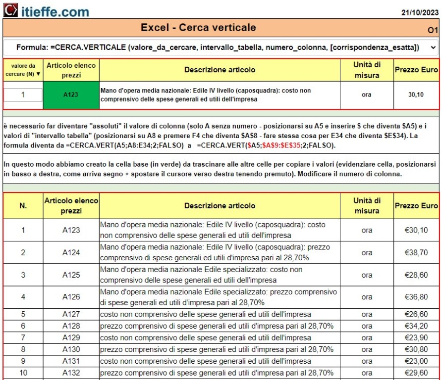
=VERTICALLOOKUP (value_to_lookup, table_range, column_number, [exact_match])
VALUE_TO_SEARCH: this is the value you want to search for within the table.
-
- TABLE_RANGE: it is the range of cells that contains the data in which you want to search for the specific value. This range must include the column in which you will look for the value and the column from which you want to extract a matching value.
- COLUMN_NUMBER: Specifies which column of the table_range contains the value you want to return. The column number is an integer that represents the position of the column within the table_range.
- [EXACT_MATCH] (optional): This argument can be “TRUE” or “FALSE”. If it is “FALSE,” Excel looks for an exact match of the value you are looking for. If it is “TRUE” or omitted, Excel looks for an approximate match or the closest value.
2 – Operation: When using the “vertical search” function, Excel searches for the specific value within the first column of the table_range. Once the matching or closest value is found (depending on the options chosen), the function returns the value from the specified column (column_number) in the same row.
3 – Example: Suppose we have a table that lists various products placed in a single row spanning various columns. If we want to find a specific value, we can use the “vertical search” function. For example:
=VLOOKUP(“X”, A11:B37, 2, FALSE).
In this case, Excel will look for “X” in the first column of the range A11:B37, and return the corresponding value from the second column.
The “vertical search” function is extremely useful for managing tabular data and for automating the retrieval of information from tables in Excel sheets. It can be used in a variety of contexts, such as inventory management, cost calculation, or creating reports based on tabular data.
Please note:
it is necessary to make the column value "absolute" (only A without number - insert $ before A which becomes $ A5) and the “table interval” values (position yourself on A11 e to press F4 which becomes $ A $ 11 – do the same thing for E37 which becomes $E$37).
The formula varies from
=VLOOKUP(A5,A11:E37,FALSE)
a
=VLOOKUP($A5;$A$11:$E$37;2;FALSE).
itieffe.com >>> Watch the video ▼
Other free programs of the same kind offered by itieffe ▼
Excel – Search Vertical
The program below is free to use.
From the reserved area it is possible to download the Microsoft Excel version of the file from which to copy all the formulas.
To access the reserved version (see below), full page and without advertising, you must be registered.
You can register now by clicking HERE